When I first read the Coconut paper1 in 2024, I got interested immediately. Their idea is simple: for the intermediate thinking process, you no longer send one token at a time; instead, you feed the model’s own output into the next token’s position, acting as an embedding. Therefore, the model can think in the latent vector space. As a neuroscientist, I’d definitely agree that we think in the latent space, aka the brain, instead of just in words, so how could I not like it? However, the authors acknowledge in the paper that their successful model, though thinking with vectors, was trained with a curriculum that is human-generated, and they tried the ideal case without human supervision, i.e., just questions and answers, but they failed. Since then, this question has kept coming back to me: if a model only sees the final answer, can it develop its own reasoning, in the latent space? I know GRPO and many of its RL descendants do, but I want more of an SFT-like solution.
At the same time, people started to question the reasoning-in-words paradigm, because they found parts of a chain of thought (CoT) can be removed or replaced without changing the answer,2 and even filler tokens that carry no meaning sometimes help as well, on the other hand.3
Now the puzzle becomes larger: a model can “think” in words, but not always and not working as it looks on the surface, though with explicit guidance on how to think. What then is the real underlying computation mechanism? If CoT is just giving more space for the model to think, will it be more natural to derive thinking in the latent space, and then why did the end2end Coconut attempt fail?
These questions triggered me and my collaborator Zhewei to design one toy task, a tiny GPT-like transformer, and several ways of thinking that we could compare side by side to attack them.
This post walks through what we found. The details are in the paper.
A small task
Natural language tasks are too hard to analyze, so we turned to easier ones and borrowed the task from the Coconut paper. The dataset is called ProsQA, in which samples are generated by an algorithm. Each sample is a list of premises like “G is Y.”, and together the premises describe a directed acyclic graph (DAG). The question then picks a root node and two candidates, and asks which of the two the root can reach. We found the original ProsQA is not perfectly controlled; a model thus can make use of things like path length to hack the problem. We thus rebuilt it with tighter controls so that a model should answer with 50% accuracy if it does not learn the essence, and we call our version ProsQA-Ext.
If you had to solve ProsQA-Ext by hand, you would start at the root, follow every edge that leaves it, then every edge that leaves those nodes, and keep going until you run into one of the candidates. With a budget of K steps, the program is a few lines:
frontier = {root}
for step in range(K):
    frontier = {b for (a, b) in edges if a in frontier}
    if c0 in frontier: answer = c0
    if c1 in frontier: answer = c1
A good property of ProsQA-Ext is that the difficulty level is easy to control: we can tune the number of hops between the root and the answer. A model that has really learned this should not care much about depth.
Then, we train on ProsQA with 3 to 6 hop samples and then test on 7 to 12 hop samples without any further training.
Five ways to think
Next we took the same small GPTNeoX LLM and trained it from scratch in five different ways.
- Direct: the model answers right after the question, no thinking at all.
- CoT: the model first generates intermediate proofs, which are learned from the shortest chain of facts, and then starts to decode answers.
- Pause: the model gets one filler token (learnable) and repeats it 6 times before it answers.
- Full-latent: this is exactly like Coconut, but without human supervision.
- Bottleneck-latent: the same as Full-latent, except that in the answer decoding phase, the model can only see its 6 thought vectors, but not the original question and their KV-cache.
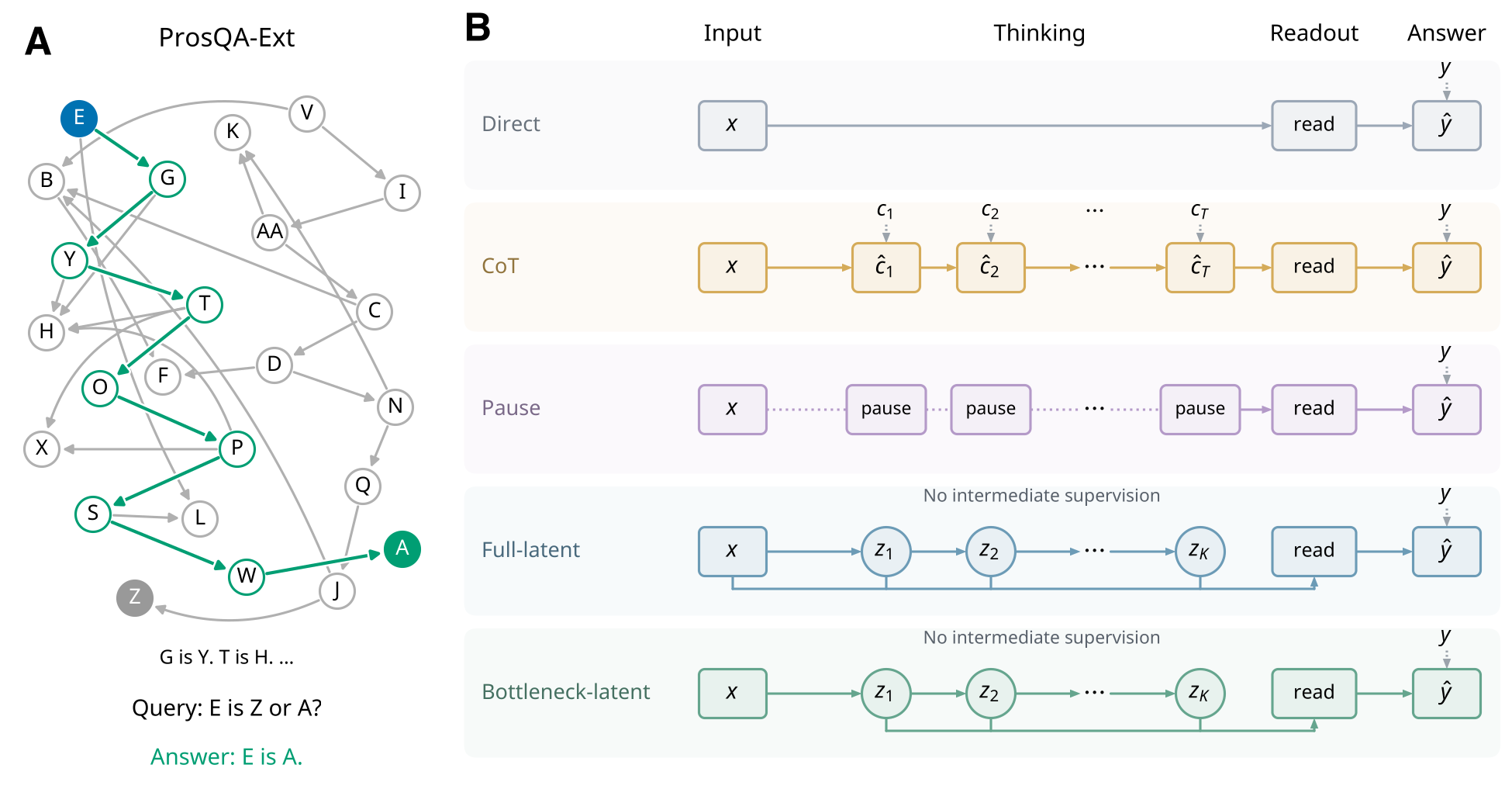
A. One 8-hop puzzle. The proof path is green and the distractor edges are gray. B. The five variants. Only the two latent models feed their own output back in, and neither gets intermediate supervision.
Same scores, until the problems get deeper
It turns out that all models pass the ID validation set, but only the two latent models perform the 7-12 OOD generalization correctly, though they received no curriculum, no reasoning traces and no RL. The bottleneck version is especially important because we wanted to isolate and understand the latent thinking without possible interference from the question. If the model cannot look back at its prompt, everything it needs for the answer has to be in the thoughts.
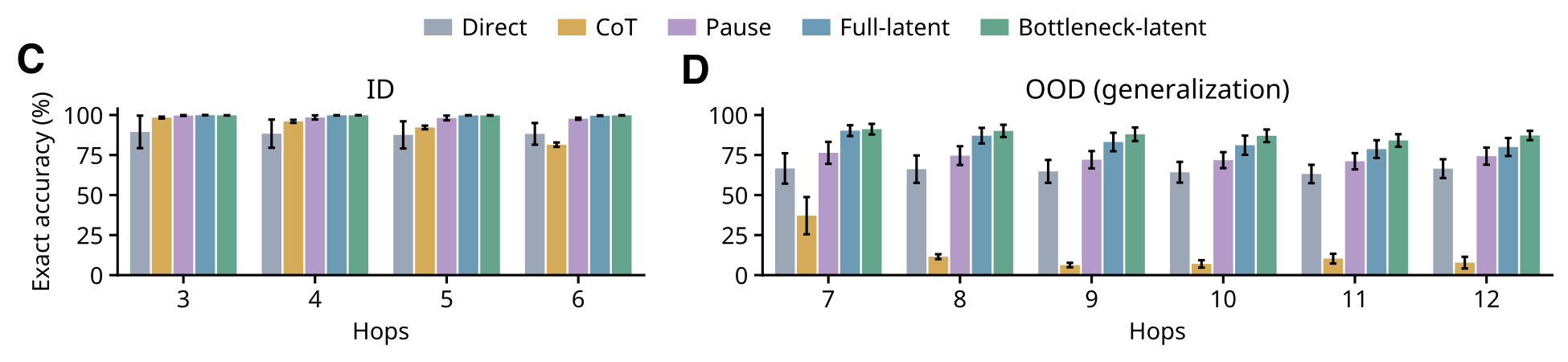
Exact-match accuracy by number of hops. C. The training range. D. Deeper problems that no model saw in training.
To our surprise, CoT performs worst and falls to about 10% once the problems have 8 hops or more. That is below chance for a question with two choices, which looks like a bug, but it is not. We found that, given a correct proof, CoT can generate correct answers. However, with free generation by exact match or a more permissive decoding strategy, it still fails.
The comparison I also find interesting here is the one with Pause. Pause has the same extra slots as the latent models and everything else is the same. In theory, this increases the expressivity of its circuit, which in practice gives it no advantage in this OOD generalization setting. So the thing that really matters in this ProsQA-Ext task is the recurrent looping mechanism in the latent space.
You may wonder why solely training on just question-answer pairs works here when it did not in Coconut. From our experiment runs it seems to be several things together: first, we found that the model size does not matter, as we replicated our results on GPT-2-small. It’s more about training sample sufficiency (the original ProsQA is too small and contains statistical bias, so a model can act like it is learning something while just fitting the superficial features) and loss design. We trained them on both the questions and answers, which helps, though this is not universal in some other tasks like arithmetic (which we also experimented with).
How do the other three get by?
This raised an obvious question. If the Direct, Pause and CoT variants fail on deeper problems, how do they solve 3 to 6 hops?
It turns out they rely on statistical shortcuts. The way the graphs are generated leaves traces in their local structure, though we tried to be very careful. For example, the correct candidate usually has a lower incoming degree than the incorrect one. We built pairs of samples that differ only in these degree statistics, and the Direct and Pause variants turned out to follow the in-degree of the candidates. Slightly differently, CoT follows the degrees of the root’s immediate successors when it chooses its first step, and its final answer goes along with that choice. In these experiments, the two latent variants are much less affected.
What the latent model is doing
So what do the latent models do instead? We looked into the bottleneck model, as all of its reasoning has to live in the six thoughts; things have to be there.
We borrowed a tool from neuroscience, representational similarity analysis (RSA). The idea is that if two DAGs have similar frontiers at depth d of the search, and the model is really tracking that frontier, then its thoughts for these two problems should be similar as well. This analysis requires no knowledge about the actual implementation, and we found that, for the latent models, the match shifts to later thoughts as d increases, as if a frontier were spreading forward from the root. We did not find such a pattern for Direct or Pause, nor for a search that runs backward from the candidates. So the models are not taking a backtracking approach.
However, RSA only shows a correlation; a real thing needs intervention. So we take a problem and swap two edges at depth d, so that the root now leads to the other candidate. We run the model on both versions, then take a single thought from the swapped run, copy it into the original run, and let the model continue its forward function from there. If the thoughts do carry the search, a swap close to the root should be able to flip the answer when we clone an early thought, and a swap deep in the DAG should only influence later thoughts. This is the exact pattern we see in the bottleneck model, and it is weaker in Full-latent and absent in Pause, further implying the existence of an iterative algorithm inside the model.
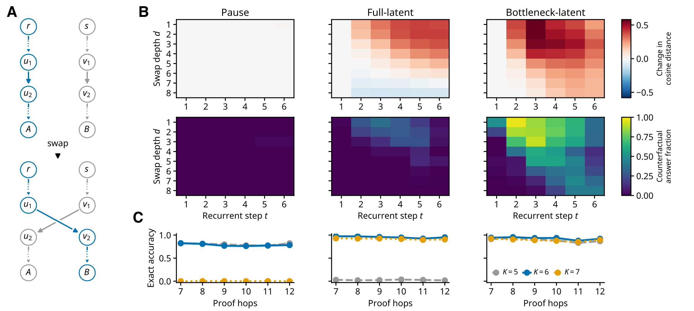
A. The edge swap. B. Top: how much a thought changes after a swap at depth d. Bottom: how often transplanting that one thought flips the answer. C. Accuracy on 7 to 12 hops when the model gets 5, 6 or 7 thoughts.
But a pebble in my shoe then persists in my mind: the bottleneck model does not fit a strict step-by-step search. We have K=6 for thinking, but the OOD has 7-12 hops. So a single thought must cover more than one hop. It made us wonder if the iterative process is really doing its job as an algorithm, so we checked this by giving the bottleneck model 5 or 7 thoughts at test time instead of six, and it preserved its accuracy. Full-latent, however, breaks with five thoughts, and Pause breaks with seven. So the loop is indeed there, but it is a soft one, where each pass moves the frontier forward by one hop or more.
This has left us more curious about the underlying mechanism of how the bottleneck works. We thus did the pruning, trimming the model to only 8 components; with these 8 alone, the pruned model agrees with the full one on about 91% of the answers.
Among these 8, we further identified two that are the ones we understand best. The first is an attention head in the last layer (L4H1), which reads the premises like a lookup table, where the key says where an edge begins and the value says where it reaches. The MLP in the same layer (L4MLP), together with the residual stream, writes the nodes that were retrieved into the next thought. Lastly, in the decoding phase, a few more heads in that layer compare the current state with the two candidates. Together, these components form a little program, in its latent space, that you may have seen above:
frontier = {root}  # carried by each thought vector
for step in range(K):
    # lookup: one attention head (key = where an edge starts, value = where it ends)
    # write:  the last MLP + residual stream put the result into the next thought
    frontier = {b for (a, b) in edges if a in frontier}
    if c0 in frontier: answer = c0  # a few heads match the state
    if c1 in frontier: answer = c1  # against the two candidates
To me, the important part is that nobody wrote this loop for the bottleneck model. What we provided is the wiring and the final answers. The step inside the loop is something the model worked out by itself.
What I take from this
Of course, this is a toy model on a toy task: four layers plus a synthetic puzzle. I do not know whether large pretrained models do anything like this, though I suspect so, as people have seen layer redundancies4 in LLMs.
We also only looked at what I would call “horizontal” recurrence, where thoughts are passed along the sequence. We’re interested in it as we want to directly compare this against those constrained to reasoning with text. I know there has been a lot of work on looped transformers5 recently, which repeat the same block in depth instead. The recurrence in depth shows its power in training because the access to the gradient is more straightforward; however, it cannot be directly related to text in our comparison, though I still think more exploration is worthwhile in these models, and I guess they may share a similar mechanism with the bottleneck-latent model.
Still, along this journey, a few things have changed in how I think about thinking in LLMs.
- LLMs with almost the same accuracy can be running very different algorithms, and we would not have noticed without rigorously designed benchmarks.
- Training a model on explicit reasoning traces did not make it reason the way we want to impose on it. CoT may work by just bridging rarely linked traces together, smoothening the process and thus getting higher accuracy.
And lastly, I have become more optimistic that there’s still room in introducing very basic primitive inductive bias into models, to induce powers like reasoning without a walking stick.
If you want the details, they are in the paper.
-
Shibo Hao, Sainbayar Sukhbaatar, DiJia Su, Xian Li, Zhiting Hu, Jason Weston, and Yuandong Tian, “Training Large Language Models to Reason in a Continuous Latent Space”, 2024. The questions-and-answers-only result is the “w/o curriculum” row of their Table 1. ↩︎
-
Tamera Lanham et al., “Measuring Faithfulness in Chain-of-Thought Reasoning”, 2023. ↩︎
-
Sachin Goyal et al., “Think before you speak: Training Language Models With Pause Tokens”, ICLR 2024; Jacob Pfau, William Merrill, and Samuel R. Bowman, “Let’s Think Dot by Dot: Hidden Computation in Transformer Language Models”, 2024. ↩︎
-
Men, Xin, et al. “ShortGPT: Layers in large language models are more redundant than you expect.” Findings of the Association for Computational Linguistics: ACL 2025. 2025. ↩︎
-
Mostafa Dehghani et al., “Universal Transformers”, ICLR 2019; Angeliki Giannou et al., “Looped Transformers as Programmable Computers”, ICML 2023. ↩︎